In my spare time I’ve been helping out my colleague Ed Evans with performance improvements to his Rust-based image processing library imgal. A few weeks ago I discovered a bug in its implementation of Kendall’s Tau coefficient. Having little statistical background, I found the source material on Kendall’s Tau, and all of its variants, rather obtuse for my brain. What I really wanted was intuition - not just the formulas that are readily available, but a clear understanding of how a coefficient is derived from the data. If such intuition exists on the internet, I couldn’t find it.

My goal with this blog post is to encapsulate the knowledge and intuition I gained about Kendall’s Tau and its variants - as such, there are sections describing the actual equations, as well as examples I crafted about my cats to build my own intuition. At the end, I also wrote a bit about how imgal actually uses Kendall’s Tau, and why the variants are necessary over its basic form. Hopefully, this saves others the investment I made into learning these algorithms.

Kendall’s Tau

Suppose you have two cats, Lucy and Penny, who each rank their four toys by preference:

Toy	Lucy	Penny
String	1	2
Ball	2	1
Laser	3	3
Mouse	4	4

Do they have similar preferences overall? As a cat owner, if they agree, you can focus on buying the types they both enjoy. If they disagree, you’ll need more variety. Measuring this kind of agreement between rankings is called rank correlation, and Kendall’s Tau coefficient is one way to quantify it.

The Formula

Kendall’s algorithm [1] compares pairs of toys. For each pair $(i, j)$, it asks: “if Lucy ranked toy $i$ better than toy $j$, did Penny also rank toy $i$ better?” If so, that pair is concording; if not, it is discording. Kendall’s Tau is:

$$\tau=\frac{(\text{number of concording pairs} - \text{number of discording pairs})}{\text{total number of pairs}}$$

This same formula appears in formal notation on Wikipedia:

$$\begin{align*} \text{Ranking 1}&=(x_1, ..., x_n) \\ \text{Ranking 2}&=(y_1, ..., y_n) \\ \tau&=\frac{2}{n(n-1)}\sum_{i\lt j}\text{sgn}(x_i-x_j)\text{sgn}(y_i-y_j). \end{align*}$$

Note the three distinct parts of this formula:

1. $\text{sgn}(x_i-x_j)\text{sgn}(y_i-y_j)$ determines if pair $(i,j)$ is concording (+1) or discording (-1)
2. $\sum_{i< j}$ sums over all unique pairs
3. The denominator $\frac{n(n-1)}{2}$ is the binomial coefficient - the total number of pairs

Note that these two formulas are really just describing the same thing. You find all unique pairs, find the difference between the number of concording and discording pairs, and divide by the total.

Example

Let’s compute Kendall’s Tau for the cats’ toy preferences. For each pair, we can determine concordance by comparing the rankings against the original table:

Pair (i, j)	Did Lucy like i better?	Did Penny like i better?	Concording?
(String, Ball)	Yes	No	No
(String, Laser)	Yes	Yes	Yes
(String, Mouse)	Yes	Yes	Yes
(Ball, Laser)	Yes	Yes	Yes
(Ball, Mouse)	Yes	Yes	Yes
(Laser, Mouse)	Yes	Yes	Yes

We have 5 concording pairs, and 1 discording pair, yielding

$$\tau=\frac{(\text{5} - \text{1})}{\text{6}}=\frac{2}{3}$$

Now that we have a value, all that is left is to map it to meaning!

Intuition

To build intuition for what different tau values mean, let’s consider three extreme scenarios.

Perfect agreement: If Lucy and Penny had identical rankings ($\text{String} \gt \text{Ball} \gt \text{Laser} \gt \text{Mouse}$), then for every pair $(i, j)$ where Lucy preferred $i$, Penny would too. All pairs concord:

$$\tau=\frac{\text{total pairs} - 0}{\text{total number of pairs}}=1$$

Perfect disagreement: If Lucy ranked the toys $\text{String} \gt \text{Ball} \gt \text{Laser} \gt \text{Mouse}$ and Penny ranked them in reverse order ($\text{Mouse} \gt \text{Laser} \gt \text{Ball} \gt \text{String}$), every pair would discord:

$$\tau=\frac{0-\text{total pairs}}{\text{total number of pairs}}=-1$$

Independence: What if Penny ranked the toys randomly, with no relation to Lucy’s preferences? On average, she’d agree with Lucy on half the pairs and disagree on the other half, giving:

$$\tau \approx \frac{\frac{\text{total pairs}}{2}-\frac{\text{total pairs}}{2}}{\text{total number of pairs}}=0$$

From these edge cases, we can see:

1. $-1\le \tau\le1$ (tau is always bounded)
2. Tau values close to $1$ indicate positive correlation (similar preferences)
3. Tau values close to $-1$ indicate negative correlation (opposite preferences)
4. Tau values close to $0$ indicate no correlation (unrelated rankings)

Hopefully, with some basic intuition about Kendall’s Tau, we can now understand some important variants!

Kendall’s Tau B

There are many situations where rankings have ties. Consider the case where Lucy cannot decide whether she likes the String or the Ball better. In fact, they’re tied for her new favorite toy:

Toy	Lucy	Penny
String	1	2
Ball	1	1
Laser	3	3
Mouse	4	4

Now, if we consider all of those $(i, j)$ toy pairs, there’s one pair where we cannot answer whether Lucy liked it better. Such tied pairs are neither concording nor discording, and do not fit cleanly into the Kendall’s Tau formula!

Pair (i, j)	Did Lucy like i better?	Did Penny like i better?	Concording?
(String, Ball)	Tied	No	Lucy Tied
(String, Laser)	Yes	Yes	Yes
(String, Mouse)	Yes	Yes	Yes
(Ball, Laser)	Yes	Yes	Yes
(Ball, Mouse)	Yes	Yes	Yes
(Laser, Mouse)	Yes	Yes	Yes

Some implementations of Kendall’s Tau use non-deterministic methods to break any ties (using, for example, Fisher-Yates shuffling [2]) but for scientific applications we require a reproducible approach.

The Formula

Fortunately, Kendall later amended his tau coefficient to encapsulate these cases [3] in a deterministic way. Since ties neither concord nor discord, they’re naturally excluded from the numerator. The denominator, however, incorporates new terms ($n_x$ and $n_y$) to account for ties. Today, this version is called $\tau_B$ (although he originally called it $\tau_s$):

$$\begin{align*} c&= \text{number of concording pairs} \\ d&= \text{number of discording pairs} \\ n&=\text{total number of pairs} \\ n_x&= \text{pairs tied in X} \\ n_y&= \text{pairs tied in Y} \\ \tau_B&=\frac{(c-d)}{\sqrt{(n-n_x)(n-n_y)}} \end{align*}$$

Note the key differences from basic Kendall’s Tau:

1. $n_x$ counts pairs that are tied in the first ranking (Lucy’s rankings in our example)
2. $n_y$ counts pairs that are tied in the second ranking (Penny’s rankings in our example)
3. The denominator $\sqrt{(n-n_x)(n-n_y)}$ normalizes the sum by the geometric mean of non-tied pairs in each ranking

Let’s see how this works with our cat toy example.

Example

For our example where Lucy created a tie, we can compute the $\tau_B$:

$$\begin{align*} c&= 5 \\ d&= 0 \\ n&= 6 \\ n_x&=1 \\ n_y&=0 \\ \tau_B&=\frac{(5-0)}{\sqrt{(6-1)(6-0)}}=\frac{5}{\sqrt{(5\times 6)}}\approx0.913 \end{align*}$$

With $\tau_B \approx 0.913$, the cats show strong agreement in their toy rankings. Notice this is higher than the original Kendall’s Tau of $\frac{2}{3} \approx 0.667$ from our first example: Lucy’s tie on $(\text{String}, \text{Ball})$ removed an explicit disagreement, bringing the rankings closer to perfect agreement.

Intuition

The denominator’s construction becomes clearer when we examine how it behaves in different scenarios:

1. Penny also liked the Ball and String equally. Imagine Penny came around to Lucy’s point of view about the String and Ball being equally good:

   Toy	Lucy	Penny
   String	1	1
   Ball	1	1
   Laser	3	3
   Mouse	4	4

   Look at how this now affects $\tau_B$:

   $$\begin{align*} c&= 5 \\ d&= 0 \\ n&= 6 \\ n_x&=1 \\ n_y&=1 \\ \tau_B&=\frac{(5-0)}{\sqrt{(6-1)(6-1)}}=\frac{5}{\sqrt{(5\times 5)}}=1 \end{align*}$$

   Now that Penny agrees with Lucy on the tie, the correlation has increased! In other words, agreement on ties is still positive correlation.

2. Penny has a tie elsewhere. Maybe Penny decides one day that the Laser is just as good as the String:

   Toy	Lucy	Penny
   String	1	2
   Ball	1	1
   Laser	3	2
   Mouse	4	4

   Now, if we’d write out the pair table, we’d find two pairings that are tied. $(String, Ball)$ is tied for Lucy, and $(String, Laser)$ is tied for Penny. Look at how this now affects $\tau_B$:

   $$\begin{align*} c&= 4 \\ d&= 0 \\ n&= 6 \\ n_x&=1 \\ n_y&=1 \\ \tau_B&=\frac{(4-0)}{\sqrt{(6-1)(6-1)}}=\frac{4}{\sqrt{(5\times 5)}}=0.8 \end{align*}$$

   Note that the denominator is the same as scenario 1, however because she tied a different pair, the number of concording pairs has decreased, decreasing the overall correlation. It’s clear that $\tau_B$ doesn’t just care about how many ties there are, but how many different pairs are affected!

3. Lucy liked everything the same. One day Lucy decides every toy is wonderful and they should all be played with equally:

   Toy	Lucy	Penny
   String	1	2
   Ball	1	1
   Laser	1	3
   Mouse	1	4

   Now, if we’d write out the pair table, we’d find all pairings are tied for Lucy. To compute correlation you need a ranking, and one of our cats has declined to do so. As such, correlation is not possible, and $\tau_B$ of course will explode:

   $$\begin{align*} c&= 0 \\ d&= 0 \\ n&= 6 \\ n_x&=6 \\ n_y&=0 \\ \tau_B&=\frac{(0-0)}{\sqrt{(6-6)(6-0)}}=\frac{0}{\sqrt{0}} \end{align*}$$

   This is different from $\tau=0$, which we saw earlier indicates independent rankings. Here, $\tau_B$ is undefined because one cat hasn’t actually ranked anything - you can’t measure correlation without a ranking. The fact that $\tau_B$ is undefined in this case is actually a feature of the metric, because it differentiates between “no correlation” and “no ranking.”

4. Almost fully tied. Note how there is a little correlation to be found if there were one different value in the ranking:

   Toy	Lucy	Penny
   String	1	2
   Ball	1	1
   Laser	1	3
   Mouse	4	4

   Now, if we’d write out the pair table, we’d find only three pairs are tied for Lucy. The other three pairs, $(String, Mouse)$, $(Ball, Mouse)$, and $(Laser, Mouse)$, are concording - both cats like the former better, and we have

   $$\begin{align*} c&= 3 \\ d&= 0 \\ n&= 6 \\ n_x&=3 \\ n_y&=0 \\ \tau_B&=\frac{(3-0)}{\sqrt{(6-3)(6-0)}}=\frac{3}{\sqrt{18}}\approx0.7 \end{align*}$$

   Intuitively, they’re more positively correlated than anything else, because they agree on the worst toy. Great!

From these scenarios, we see that the denominator $\sqrt{(n-n_x)(n-n_y)}$ elegantly handles rankings with ties: agreement on ties is rewarded (scenario 1) but disagreement is penalized (scenario 2). It provides an intuitive outcome for all-tied rankings (scenario 3), and mostly-tied rankings (scenario 4). Let’s look at another variant!

Weighted Kendall’s Tau

It’s common in statistics to put more emphasis on particular indices within the rankings. For example, I might want to weight my cats’ toy rankings by how long they’ve played with each toy. A cat who’s spent months with a toy knows it brand new and after heavy use—their ranking is more reliable than for a toy they got yesterday.

The Formula

Kendall himself didn’t address weighting, but Grace Shieh did years later [4]. Using notation akin to the unweighted Kendall’s Tau:

$$\begin{align*} \text{Ranking 1}&=(x_1, ..., x_n) \\ \text{Ranking 2}&=(y_1, ..., y_n) \\ \text{Weights}&=(v_1, ..., v_n) \\ \tau_w&=\frac{\sum_{i\lt j}v_iv_j\text{sgn}(x_i-x_j)\text{sgn}(y_i-y_j)}{\frac{1}{2}((\sum_{i}v_i)^2-\sum_{i}v_i^2)} \end{align*}$$

The formula is similar to unweighted $\tau$, but each pair $(i,j)$ gets multiplied by its pair weight $v_iv_j$. Shieh’s original formulation uses a general weight function $w_{ij}$ that can depend on both indices, which is useful for more complex weighting schemes [5], but many implementations only support index weights as shown above.

Example

Let’s go back to our example with Lucy and Penny. Suppose they’ve spent 10 hours with the String, 8 hours with the Ball, 2 hours with the Laser, and just 1 hour with the Mouse. I could use these as weights to refine their rank correlation:

Toy	Lucy	Penny	Weight
String	1	2	10
Ball	2	1	8
Laser	3	3	2
Mouse	4	4	1

We now can multiply the weights to get a weight value for each pair:

Pair (i, j)	Did Lucy like i better?	Did Penny like i better?	Concording?	Pair Weight = $w_i*w_j$
(String, Ball)	Yes	No	No	80
(String, Laser)	Yes	Yes	Yes	20
(String, Mouse)	Yes	Yes	Yes	10
(Ball, Laser)	Yes	Yes	Yes	16
(Ball, Mouse)	Yes	Yes	Yes	8
(Laser, Mouse)	Yes	Yes	Yes	2

The weighted Kendall’s Tau would add the weights of all of the concording pairs, subtract the weights of all of the discording pairs, and then divide by the sum of all of the weights:

$$\tau_w=\frac{(20+10+16+8+2) - 80}{(80+20+10+16+8+2)}=\frac{56-80}{136}\approx-0.176$$

Intuition

The weighted version mirrors the unweighted version with two key changes:

1. Numerator: Each pair gets multiplied by its pair weight $v_iv_j$ instead of counting as 1.
2. Denominator: We sum all pair weights ($\sum_{i\ne j} v_iv_j = \frac{1}{2}((\sum_iv_i)^2-\sum_iv_i^2)$) instead of counting pairs.

The dramatic flip from $\tau=\frac{2}{3}$ to $\tau_w\approx -0.176$ shows the power of weighting. String vs Ball was the only discording pair, but it had the highest pair weight (80) because both toys were played with extensively. That single heavily-weighted disagreement outweighed all five concording pairs combined (sum of 56). When toys are weighted by play time, Lucy and Penny’s disagreement on their two favorite toys dominates the correlation.

What about ties?

Weighted Kendall’s Tau B

Weighted Kendall’s Tau B combines both extensions: handling ties and using weights. The key intuitions remains the same—instead of summing over pairs, we sum over pair weights, and we alter the denominator to account for ties.

The Formula

Consider the unweighted Kendall’s Tau B:

$$\begin{align*} c&= \text{number of concording pairs} \\ d&= \text{number of discording pairs} \\ n&= \text{total number of pairs} \\ n_x&= \text{pairs tied in X} \\ n_y&= \text{pairs tied in Y} \\ \tau_B&=\frac{(c-d)}{\sqrt{(n-n_x)(n-n_y)}} \end{align*}$$

To write a weighted version $\tau_{wB}$, all we need to do is replace pairs with pair weights. Let’s use $w$ subscripts to distinguish from the unweighted version:

$$\begin{align*} c_w&= \text{sum of concording pair weights} \\ d_w&= \text{sum of discording pair weights} \\ n_w&= \text{sum of all pair weights} \\ n_{wx}&= \text{sum of pair weights tied in X} \\ n_{wy}&= \text{sum of pair weights tied in Y} \\ \tau_{wB}&=\frac{(c_w-d_w)}{\sqrt{(n_w-n_{wx})(n_w-n_{wy})}} \end{align*}$$

Example

One final example. Lucy again decides she likes the Ball and the String equally, after 10 hours of play with the String, 8 hours of play with the Ball, 2 hours of play with the Laser, and an hour of play with the Mouse:

Toy	Lucy	Penny	Weight
String	1	2	10
Ball	1	1	8
Laser	3	3	2
Mouse	4	4	1

Recall that unweighted $\tau_B=0.913$ was higher than unweighted $\tau=\frac{2}{3}$ because Lucy’s tie removed the explicit disagreement, bringing the rankings closer to total agreement.

We’d expect the same pattern here: weighted $\tau_{wB}$ should be higher than weighted $\tau_w\approx -0.176$ because we’re removing that heavily-weighted String vs Ball disagreement. Let’s compute the pair weights:

Pair (i, j)	Did Lucy like i better?	Did Penny like i better?	Concording?	Pair Weight = $w_i*w_j$
(String, Ball)	Tied	No	Lucy Tied	80
(String, Laser)	Yes	Yes	Yes	20
(String, Mouse)	Yes	Yes	Yes	10
(Ball, Laser)	Yes	Yes	Yes	16
(Ball, Mouse)	Yes	Yes	Yes	8
(Laser, Mouse)	Yes	Yes	Yes	2

Using this table, we can compute the weighted Kendall’s Tau B:

$$\begin{align*} c_w&= 20 + 10 + 16 + 8 + 2 = 54 \\ d_w&= 0 \\ n_w&= 80 + 20 + 10 + 16 + 8 + 2 = 136 \\ n_{wx}&= 80 \\ n_{wy}&= 0 \\ \tau_{wB}&=\frac{(c_w-d_w)}{\sqrt{(n_w-n_{wx})(n_w-n_{wy})}}=\frac{(54-0)}{\sqrt{(136-80)(136-0)}}\approx0.619 \end{align*}$$

As expected, $\tau_{wB}\approx 0.619$ is much higher than $\tau_w\approx -0.176$. The tie neutralized the heavily-weighted disagreement that dominated the weighted calculation, revealing the underlying positive correlation in the remaining pairs.

Finale: The Use Case

As I mentioned at the beginning of this post, I’ve been helping my colleague clean up imgal’s implementation of Weighted Kendall’s Tau B. This metric is a key component of Spatially Adaptive Colocalization Analysis (SACA), a colocalization framework developed by Shulei Wang and our former colleague Ellen Arena [6]. Unlike many of its alternatives, it doesn’t require a human (or AI!) to designate a region of interest and accounts for the spatial characterstics of the data. Programmatic SACA implementations aren’t widely available, so providing a fast, well-documented, and open implementation was one of the core motivations for the creation of imgal.

Colocalization metrics like SACA help scientists quantify how different cellular markers (e.g. fluorescent fusion proteins) correlate and/or co-occur spatially within a sample. To do this, biologists capture multi-channel images of a sample, where each channel excites a different fluorescent target. By quantifying whether (and where) those fluorescent targets colocalize, we can better understand the captured markers’ biological relationships—whether proteins interact, whether cellular processes are coordinated, or whether disease markers cluster together.

To compute colocalization strength, SACA derives rankings for each location in the channel images, and then uses Weighted Kendall’s Tau B to compute a colocalization coefficient. These rankings come from the intensities in a circular neighborhood around each location. Candidate pixels farther away from the center of the neighborhood say less about colocalization than closer neighbors, so SACA uses a weighted Kendall’s Tau, with weights decaying towards the edge of the circle.

In addition, SACA requires a tie-handling variant of Kendall’s Tau because microscopy cameras typically produce images of 16-bit unsigned integers. With a 512x512 image, the pigeonhole principle guarantees some pixels in the image have the same intensity, and they could end up being close together.

SACA is iterative, computing Weighted Kendall’s Tau B for every pixel, multiple times until convergence. A 1024x1024 image means over a million correlation calculations per iteration, making it the performance bottleneck of imgal’s implementation.

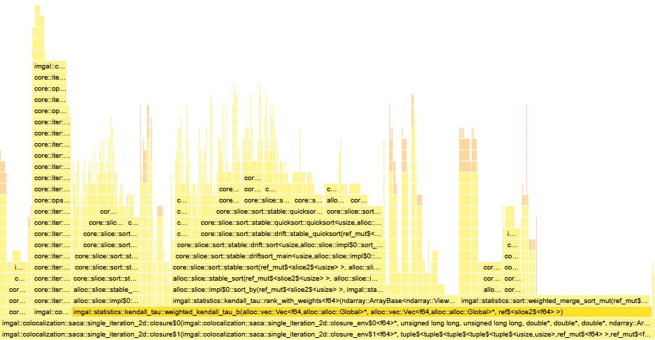
To make SACA viable for real biological research, we are motivated to make our Kendall’s Tau implementations fast (and, of course, correct!), and to do that, we must understand all of the algorithm’s variants. As such, I’ve recorded my understanding here—understanding that will hopefully lead to a correct, efficient SACA implementation in imgal.

Acknowledgements

Thanks to my colleague Ed Evans for reviewing this draft and providing valuable technical insights on SACA and colocalization analysis. His feedback greatly improved the accuracy of this post.

References

[1] https://doi.org/10.1093%2Fbiomet%2F30.1-2.81

[2] https://github.com/scijava/scijava/blob/13f00a282b10cddc79846617e2ec4618628fc60a/scijava-ops-image/src/main/java/org/scijava/ops/image/coloc/saca/WtKendallTau.java#L136-L143

[3] https://doi.org/10.2307%2F2332303

[4] https://doi.org/10.1016/S0167-7152(98)00006-6

[5] https://doi.org/10.1145/2736277.2741088

[6] https://doi.org/10.1109/tip.2019.2909194

---